NN training

This section is an excerpt from the notebook explaining how to train a cosmopower_NN model. The user is strongly encouraged to run that notebook in its entirety, . Here we will consider only the most important parts to understand how the training works.

PARAMETER FILES¶

Let’s take a look at the content of the parameter files that are read by CosmoPower during training.

training_parameters = np.load('./camb_tt_training_params.npz')

training_parameters is a dict of np.arrays. There is a dict key for each of the parameters the emulator will be trained on:

print(training_parameters.files)

['omega_b', 'omega_cdm', 'h', 'tau_reio', 'n_s', 'ln10^{10}A_s']

Each of these keys has a np.array of values: the number of elements in the array is the number of training samples in our set. For example:

print(training_parameters['omega_b'])
print('number of training samples: ', len(training_parameters['omega_b'])) # same for all of the other parameters

[0.03959524 0.03194429 0.03467569 ... 0.03958164 0.02816863 0.01942146]
number of training samples:  42614

FEATURE FILES¶

Now let’s take a look at the “features”. With features here we refer to the predictions of the neural network: these may be spectra or log-spectra values. For example, in this notebook we are emulating values of the TT log-power spectra. These are sampled at each multipole \(\ell\) in the range \([2, \dots 2508]\), hence our training sample for each log-spectrum will be a 2507-dimensional array. The corresponding .npz files contain a dict with two keys:

training_features = np.load('./camb_tt_training_log_spectra.npz')
print(training_features.files)

['modes', 'features']

The first key, modes, contains a np.array of the sampled Fourier modes (multipoles, in this CMB case):

print(training_features['modes'])
print('number of multipoles: ', len(training_features['modes']))

[   2    3    4 ... 2506 2507 2508]
number of multipoles:  2507

The second key, features, has values equal to the actual values of the log-spectra. These are collected in a np.array of shape (number of training samples, number of Fourier modes):

training_log_spectra = training_features['features']
print('(number of training samples, number of ell modes): ', training_log_spectra.shape)

(number of training samples, number of ell modes):  (42614, 2507)

The files for the testing samples have the same type of content.

testing_params = np.load('./camb_tt_testing_params.npz')
testing_spectra = 10.**(np.load('./camb_tt_testing_log_spectra.npz')['features'])

`cosmopower_NN` INSTANTIATION¶

We will now create an instance of the cosmopower_NN class.

In order to instantiate the class, we need to first define some of the key aspects of our model.

PARAMETERS¶

Let’s start by defining the parameters of our model. cosmopower_NN will take in input a set of these parameters for each prediction.

If, for example, we want to emulate over a set of 6 standard \(\Lambda\)CDM parameters,

\(\omega_{\mathrm{b}}, \omega_{\mathrm{cdm}}, h, \tau, n_s, \ln10^{10}A_s\)

we need to create a list with the names of all of these parameters, in arbitrary order:

model_parameters = ['h', 
                    'tau_reio', 
                    'omega_b', 
                    'n_s', 
                    'ln10^{10}A_s', 
                    'omega_cdm', 
                    ]

This list will be sent in input to the cosmopower_NN class, which will use this information:

to derive the number of parameters in our model, equal to the number of elements in model_parameters. This number also corresponds to the number of nodes in the input layer of the neural network;
to free the user from the burden of having to manually perform any ordering of the input parameters.

The latter point guarantees flexibility and simplicity while using cosmopower_NN: to obtain predictions for a set of parameters, the user simply needs to feed a Python dict to cosmopower_NN, without having to worry about the ordering of the input parameters.

For example, if I wanted to know the neural network prediction for a single set of parameters, I would collect them in the following dict:

example_single_set_input_parameters = {'n_s': [0.96], 
                                       'h': [0.7], 
                                       'omega_b': [0.0225], 
                                       'omega_cdm': [0.13], 
                                       'tau_reio': [0.06], 
                                       'ln10^{10}A_s': [3.07], 
                                        }

Similarly, if I wanted to ask cosmopower_NN for e.g. 3 predictions, for 3 parameter sets, I would use:

example_multiple_sets_input_parameters = {'n_s': np.array([0.96, 0.95, 0.97]), 
                                          'h': np.array([0.7, 0.64, 0.72]), 
                                          'omega_b': np.array([0.0225, 0.0226, 0.0213]), 
                                          'omega_cdm': np.array([0.11, 0.13, 0.12]), 
                                          'tau_reio': np.array([0.07,0.06, 0.08]), 
                                          'ln10^{10}A_s': np.array([2.97, 3.07, 3.04]), 
                                           }

The possibility of asking cosmopower_NN for batch predictions, in particular, makes it a particularly useful tool to integrate within samplers that allow for batch evaluations of the likelihood.

MODES¶

A second, important piece of information for the cosmopower_NN class is the number of its output nodes, which corresponds to the number of sampled Fourier modes in our (log)-spectra, i.e. the number of multipoles \(\ell\) for the CMB spectra, or the number of \(k\)-modes for the matter power spectrum.

In the example of this notebook, we will emulate all of the \(\ell\) multipoles between 2 and 2508. Note that we exclude \(\ell=0,1\) as these are always 0. We can read the sampled \(\ell\) range from the modes entry of our training_features dict (previously loaded):

ell_range = training_features['modes']
print('ell range: ', ell_range)

ell range:  [   2    3    4 ... 2506 2507 2508]

CLASS INSTANTIATION¶

Finally, let’s feed the information on model parameters and number of outputs to the cosmopower_NNclass, which we instantiate with the following:

from cosmopower import cosmopower_NN

cp_nn = cosmopower_NN(parameters=model_parameters, 
                      modes=ell_range, 
                      n_hidden = [512, 512, 512, 512], # 4 hidden layers, each with 512 nodes
                      verbose=True, # useful to understand the different steps in initialisation and training
                      )

Initialized cosmopower_NN model, 
mapping 6 input parameters to 2507 output modes, 
using 4 hidden layers, 
with [512, 512, 512, 512] nodes, respectively.

TRAINING¶

This section shows how to train our model.

To do this, we will call the method train() from the cosmopower_NN class. Here are the input arguments for this function:

training_parameters: as explained above, this is a dict of np.arrays of input parameters. Each dict key has a np.array of values, for example

training_parameters = {`omega_b` : np.array([0.0222, 0.0213, 0.0241, ...]),
                       `omega_cdm` : np.array([0.114, 0.134, 0.124, ...]),
                        ... etc ...
                      }

(each np.array has the same number of elements, equal to the number of training samples);

training_features: a np.array of training (log)-power spectra. Its dimensions are (number of training samples, number of Fourier modes);
filename_saved_model: path (without suffix) to the .pkl file where the trained model will be saved;
validation split: float between 0 and 1, percentage of samples from the training set that will be used for validation.

Some of the input arguments allow for the implementation of a learning schedule with different steps, each characterised by a different learning rate. In addition to the learning rate, the user can change other hyperparameters, such as the batch size, at each learning step:

learning_rates: list of float values, the optimizer learning rate at each learning step;
batch_sizes: list of float values, batch size for each learning step;
gradient_accumulation_steps: list of int values, the number of accumulation batches if using gradient accumulation, at each learning step. Set these numbers to > 1 to activate gradient accumulation - only worth doing if using very large batch sizes;
patience_values: list of int values, the number of epochs to wait for early stopping, at each learning step;
max_epochs: list of int values, the maximum number of epochs for each learning step.

with tf.device(device):
    # train
    cp_nn.train(training_parameters=training_parameters,
                training_features=training_log_spectra,
                filename_saved_model='TT_cp_NN_example',
                # cooling schedule
                validation_split=0.1,
                learning_rates=[1e-2, 1e-3, 1e-4, 1e-5, 1e-6],
                batch_sizes=[1024, 1024, 1024, 1024, 1024],
                gradient_accumulation_steps = [1, 1, 1, 1, 1],
                # early stopping set up
                patience_values = [100,100,100,100,100],
                max_epochs = [1000,1000,1000,1000,1000],
                )

After running this cell, the model is trained and, if we are satisfied with its performance on the testing set (see next section), we can download the .pkl file where the model was saved (given by the filename_saved_model argument of the train method of the cosmopower_NN class).

TESTING¶

To compute the predictions of the trained model on the testing set, we start by loading the trained model

cp_nn = cosmopower_NN(restore=True, 
                      restore_filename='TT_cp_NN_example',
                      )

Let’s compute the predictions for the testing parameters. Note that we use the function ten_to_predictions_np, which, given input parameters,

first performs forward passes of the trained model
and then computes 10^ these predictions.

Since we trained our model to emulate log-spectra, the output of ten_to_predictions_np is then given by predicted spectra.

NOTE 1: If we had trained our model to emulate spectra (without log), then to obtain predictions we would have used the function predictions_np.

NOTE 2: the functions ten_to_predictions_np and predictions_np implement forward passes through the network using only Numpy. These are optimised to be used in pipelines developed in simple Python code (not pure-Tensorflow pipelines).

Conversely, the functions ten_to_predictions_tf and predictions_tf are pure-Tensorflow implementations, and as such are optimised to be used in pure-Tensorflow pipelines.

NOTE 3: both pure-Tensorflow and Numpy implementations allow for batch evaluation of input parameters - here, in particular, we can obtain predictions for all of the testing_parameters in just a single batch evaluation.

predicted_testing_spectra = cp_nn.ten_to_predictions_np(testing_params)

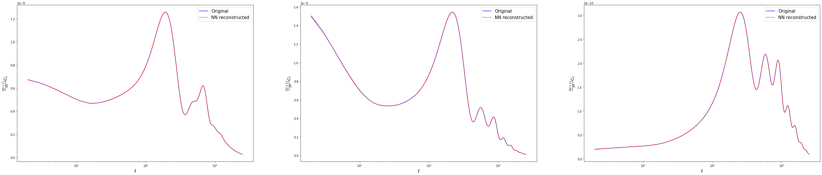
Plot examples of power spectra predictions from the testing set

from matplotlib import gridspec
fig, ax = plt.subplots(nrows=1, ncols=3, figsize=(50,10))
for i in range(3):
    pred = predicted_testing_spectra[i]*ell_range*(ell_range+1)/(2.*np.pi)
    true = testing_spectra[i]*ell_range*(ell_range+1)/(2.*np.pi)
    ax[i].semilogx(ell_range, true, 'blue', label = 'Original')
    ax[i].semilogx(ell_range, pred, 'red', label = 'NN reconstructed', linestyle='--')
    ax[i].set_xlabel('$\ell$', fontsize='x-large')
    ax[i].set_ylabel('$\\frac{\ell(\ell+1)}{2 \pi} C_\ell$', fontsize='x-large')
    ax[i].legend(fontsize=15)

png

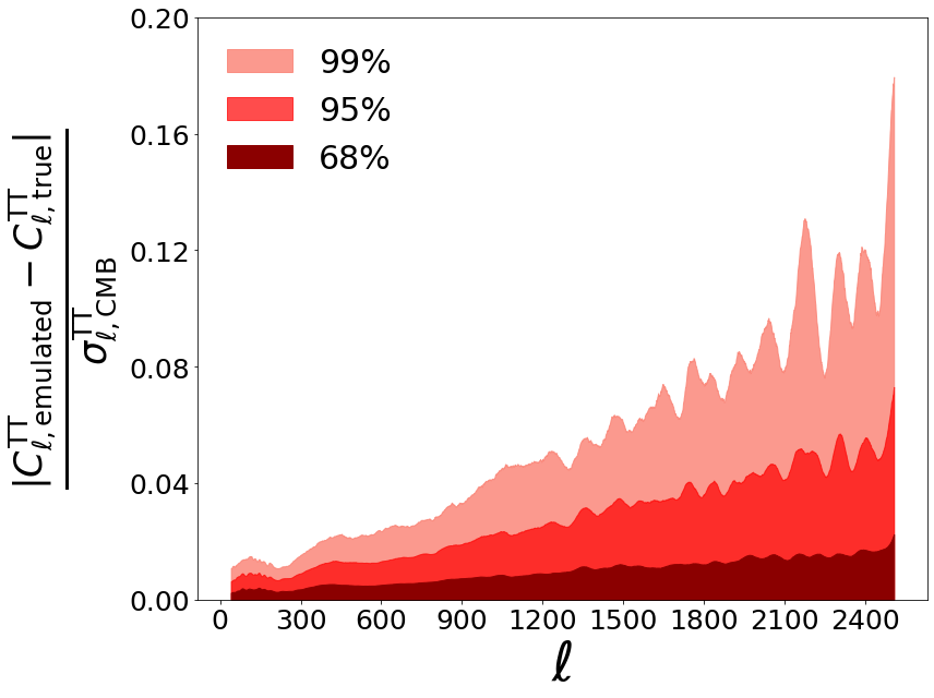
We want to plot accuracy in units of Simons Observatory (SO) noise curves. Start by loading SO noise curves from the SO repository

!git clone https://github.com/simonsobs/so_noise_models

noise_levels_load = np.loadtxt('./so_noise_models/LAT_comp_sep_noise/v3.1.0/SO_LAT_Nell_T_atmv1_goal_fsky0p4_ILC_CMB.txt')
conv_factor = (2.7255e6)**2

ells = noise_levels_load[:, 0]
SO_TT_noise = noise_levels_load[:, 1][:2509-40] / conv_factor
new_ells = ells[:2509-40]

f_sky = 0.4
prefac = np.sqrt(2/(f_sky*(2*new_ells+1)))
denominator = prefac*(testing_spectra[:, 38:]+SO_TT_noise)  # use all of them
diff = np.abs((predicted_testing_spectra[:, 38:] - testing_spectra[:, 38:])/(denominator))

percentiles = np.zeros((4, diff.shape[1]))

percentiles[0] = np.percentile(diff, 68, axis = 0)
percentiles[1] = np.percentile(diff, 95, axis = 0)
percentiles[2] = np.percentile(diff, 99, axis = 0)
percentiles[3] = np.percentile(diff, 99.9, axis = 0)

plt.figure(figsize=(12, 9))
plt.fill_between(new_ells, 0, percentiles[2,:], color = 'salmon', label = '99%', alpha=0.8)
plt.fill_between(new_ells, 0, percentiles[1,:], color = 'red', label = '95%', alpha = 0.7)
plt.fill_between(new_ells, 0, percentiles[0,:], color = 'darkred', label = '68%', alpha = 1)

plt.ylim(0, 0.2)

plt.legend(frameon=False, fontsize=30, loc='upper left')
plt.ylabel(r'$\frac{| C_{\ell, \rm{emulated}}^{\rm{TT}} - C_{\ell, \rm{true}}^{\rm{TT}}|} {\sigma_{\ell, \rm{CMB}}^{\rm{TT}}}$', fontsize=50)
plt.xlabel(r'$\ell$',  fontsize=50)

ax = plt.gca()
ax.xaxis.set_major_locator(plt.MaxNLocator(10))
ax.yaxis.set_major_locator(plt.MaxNLocator(5))

plt.setp(ax.get_xticklabels(), fontsize=25)
plt.setp(ax.get_yticklabels(), fontsize=25)
plt.tight_layout()

png